How To Draw A Horizontal Line In A Cell In Excel

Tuesday, September xi, 2018
Peltier Technical Services, Inc., Copyright © 2021, All rights reserved.

A common task is to add a horizontal line to an Excel chart. The horizontal line may reference some target value or limit, and adding the horizontal line makes information technology like shooting fish in a barrel to run into where values are above and below this reference value. Seems easy enough, but oftentimes the result is less than ideal. This tutorial shows how to add horizontal lines to several common types of Excel chart.

Nosotros won't even talk about trying to draw lines using the items on the Shapes menu. Since they are drawn freehand (or free-mouse), they aren't positioned accurately. Since they are independent of the nautical chart's data, they may not move when the information changes. And sometimes they but seem to move whenever they feel like it.

The examples beneath evidence how to make combination charts, where an XY-Scatter-type series is added as a horizontal line to another type of chart.

Add a Horizontal Line to an XY Scatter Nautical chart

An XY Scatter chart is the easiest case. Here is a simple XY chart.

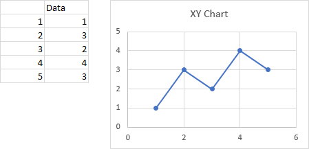
XY Scatter Chart Without Horizontal Line

Let's say we want a horizontal line at Y = two.5. Information technology should span the chart, starting at X = 0 and ending at X = 6.

This is easy, a line simply connects two points, right?

We gear up a dummy range with our initial and terminal Ten and Y values (below, to the left of the superlative chart), copy the range, select the chart, and apply Paste Special to add the data to the chart (run into below for details on Paste Special).

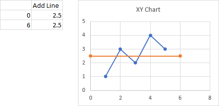
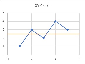
XY Scatter Chart With Ugly Horizontal Line

When the information is beginning added, the autoscaled 10 centrality changes its maximum from 6 to 8, and so the line doesn't bridge the entire chart. We take to format the axis and type six into the box for Maximum. We probably too want to remove the markers from our horizontal line.

Paste Special

If you don't employ Paste Special often, it might be difficult to find. If you lot copy a range and utilize the right click bill of fare on a chart, the but option is a regular Paste, and Excel doesn't ever correctly gauge how information technology should paste the data. So I always apply Paste Special.

To notice Paste Special, click on the down arrow on the Paste push button on the Home tab of Excel'southward ribbon. Paste Special is at the bottom of the popular-up menu.

You can besides employ the Excel 97-2003 bill of fare-based shortcut, which is Alt + E + S (for Eastdit menu > Paste Southpecial).

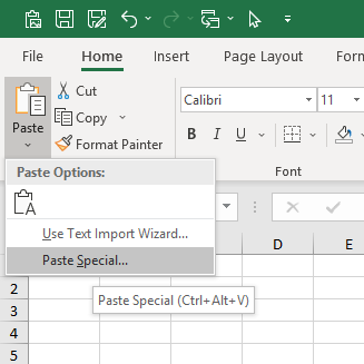
The tooltip below Paste Special in the bill of fare indicates that you could as well utilize Ctrl + Alt + 5, but this shortcut doesn't do anything for charts.

When the Paste Special dialog appears, brand sure y'all select these options: Add Cells as a New Series, Y Values in Columns, Series Names in Offset Row, Categories (X Values) in First Column.

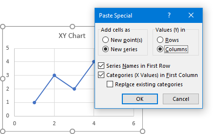
Click OK and the new serial will appear in the chart.

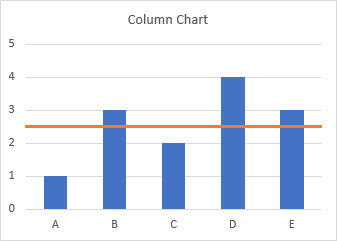
Add a Horizontal Line to a Column or Line Chart

When you add a horizontal line to a chart that is not an XY Scatter chart blazon, information technology gets a flake more complicated. Partly it'south complicated because we volition be making a combination chart, with columns, lines, or areas for our data along with an XY Scatter blazon series for the horizontal line. Partly it's complicated because the category (X) centrality of most Excel charts is not a value axis.

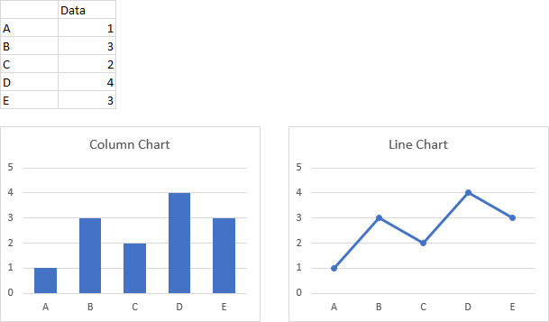
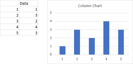
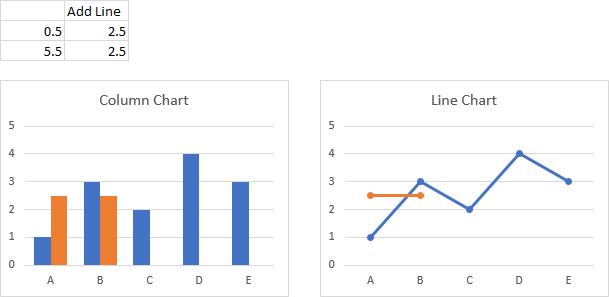
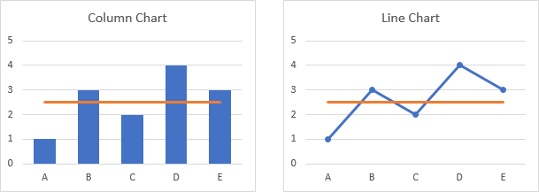
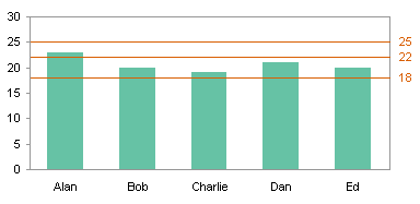
Equally with the XY Scatter chart in the offset example, we need to figure out what to apply for X and Y values for the line nosotros're going to add. The Y values are easy, merely the X values require a trivial understanding of how Excel'south category axes work. Since the category axes of cavalcade and line charts work the aforementioned way, let's do them together, starting with the following simple column and line charts.

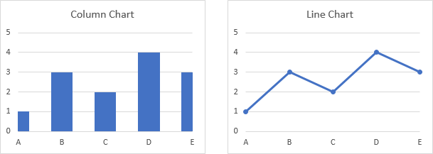
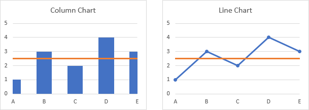
Column and Line Charts Without Horizontal Lines

Note in the charts higher up that the outset and concluding category labels aren't positioned at the corners of the plot area, only are moved in slightly. This is because column and line charts utilise a default setting of Between Tick Marks for the Axis Position holding. Nosotros can change the Axis Position to On Tick Marks, below, and the first and last category labels line upward with the ends of the category axis. The line chart looks okay, but we accept cutting off the outer halves of the outset and final columns.

Allow's focus on a column chart (the line chart works identically), and use category labels of one through 5 instead of A through E. Excel doesn't recognize these categories as numerical values, just we can think of them every bit labeling the categories with numbers.

At present allow's label the points between the categories. Not just practice we accept halfway points between the categories, we also take a half category characterization below the first category and another after the last category.

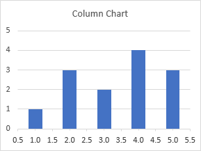
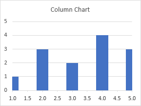
Column Chart With Categories 1-5 and Mid Categories

If the Axis Position property were fix to On Tick Marks, our horizontal line starts at i (the commencement category number of i) and ends at five (the last category number of 5). This would be wrong for a column nautical chart, but might exist acceptable for a line chart.

Column Chart With Desired Horizontal Line

Here is our desired horizontal line, stretching from 0.5 to v.5

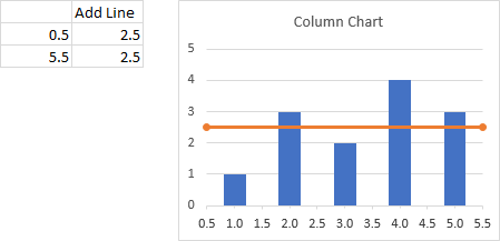
So permit's use this data and the aforementioned approach that we used for the besprinkle chart, at the starting time of this tutorial.

Copy the range, and paste special equally new series. Nosotros've added another set of columns or some other line to the chart.

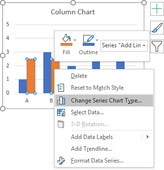
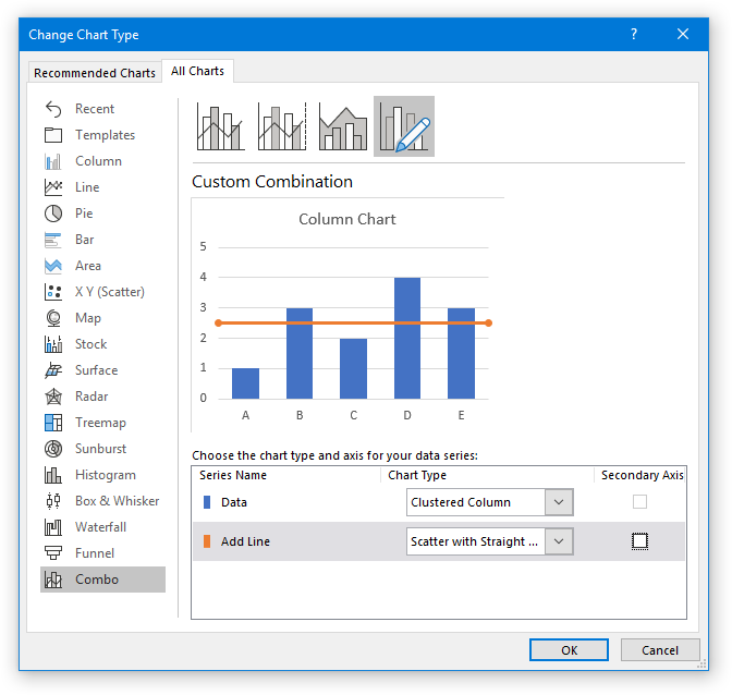
Column and Line Chart With Horizontal Line

Right click on the added series, and choose Change Serial Chart Type from the pop-upwards menu.

In the Change Chart Type dialog, select the XY Scatter With Straight Lines And Markers chart type. We're using markers to temporarily marking the ends of the line, and nosotros'll remove the markers subsequently; in general we will change directly to XY Scatter With Directly Lines.

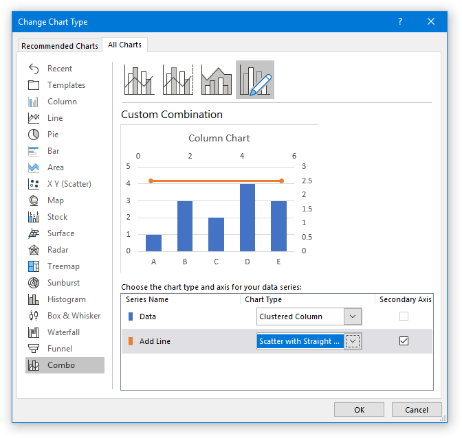
The new series don't line upward at all, though, because Excel decided nosotros should plot the scatter serial on the secondary axes. We could rescale the secondary axes, then hide them, but that makes a complicated situation even more complicated.

So we need to uncheck the Secondary Centrality box next to the Scatter serial in the Change Chart Type dialog.

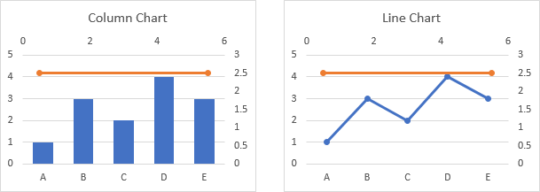
Change Series Chart Type And Axis Dialog

And now everything lines upwards as expected: the markers on the horizontal lines are at the edges of the plot area.

We should remove those markers now, and in the future select the chart type without markers.

"Lazy" Horizontal Line

You lot may ask why non make a combination cavalcade-line chart, since cavalcade charts and line charts use the same axis blazon. And many charts with horizontal lines use exactly this approach. I call it the "lazy" approach, because information technology's easier, but it provides a line that doesn't extend beyond all the information to the sides of the chart.

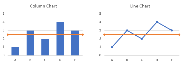
Beginning with your chart data, and add a column of values for the horizontal line. You get a column chart with a second set of columns, or a line chart with a second line.

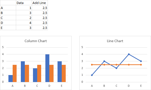
Column and Line Charts With Lazy Horizontal Lines

Modify the chart type of the added series to a line chart without markers. Doesn't look very skillful for the column chart (left) since the horizontal line ends at the centerlines of the outset and final column. You lot could probably become abroad with it for the line chart, even though the horizontal line doesn't extend to the sides of the chart.

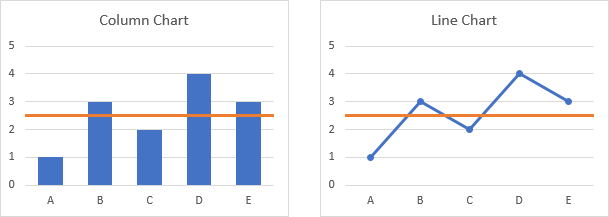
If we change the Centrality Position and then the vertical axis crosses On Tick Marks, the horizontal lines for both charts span the entire chart width. In the column chart, this comes at the expense of the outer halves of the first and last columns. The line chart looks okay, though.

Add a Horizontal Line to an Area Chart

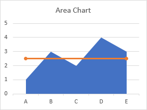
As with the previous examples, we need to figure out what to apply for X and Y values for the line nosotros're going to add. The category axis of an surface area chart works the same as the category axis of a column or line chart, but the default settings are different. Let's outset with the post-obit unproblematic area chart.

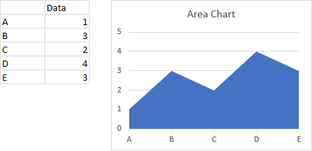
Notice that the offset and last category labels are aligned with the corners of the plot expanse and the filled area series extends to the sides of the plot area. This is because the default setting of theAxis Position property is On Tick Marks. Nosotros can change it to Between Tick Marks, which makes the area chart look a bit strange.

Beneath is the data for our horizontal line, which will first at 1 (the first category number of 1) and cease at 5 (the terminal category number of 5), without the half-category cushion at either cease. Copy the data, select the nautical chart, and Paste Special to add the data every bit a new serial.

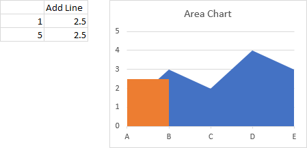
Right click on the added series, and change its nautical chart type to XY Scatter With Straight Lines And Markers (again, the markers are temporary). The resulting line extends to the edges of the plotted area, but Excel changed the Axis Position to Between Tick Marks.

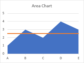
Modify the Axis Position setting back to On Tick Marks, and remove the markers from the line.

"Lazy" Horizontal Line

In the column chart, and maybe for the line chart, the "lazy" approach did not give a suitable horizontal line, since the line did not extend to the edges of the plot expanse. Let'south meet how it works for an expanse chart.

Make a chart with the actual data and the horizontal line data.

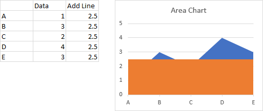
Correct click on the second serial, and change its chart type to a line. Excel changed the Axis Position property to Between Tick Marks, similar information technology did when we inverse the added series above to XY Scatter.

Modify the Axis Position dorsum to On Tick Marks, and the chart is finished.

For the expanse chart, the appearance of the lazy horizontal line is identical to the more complicated line that uses an XY Besprinkle series. Since it's easier and only as good, it's probably amend to utilize the lazy arroyo.

Follow-Up

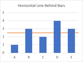
An alert reader noted in the comments that the line produced by this method is placed in front of the bars, and it might be better to place such reference lines behind the data. I have written a new post describing an approach that does merely this: Horizontal Line Backside Columns in an Excel Chart.